Types of Scheduling Algorithm in OS With Examples

A scheduling algorithm is a technique or method that is used to organize, manage and check work and workloads on a CPU. Types of scheduling algorithms are  FCFS, SJF, priority scheduling, etc. To learn more let’s read it further.

Scheduling Algorithm

Scheduling is based on the information that is available at a given time. We need some way to represent the state of the system and any processes in it and how it changes over time.

Gantt charts are used for this purpose. A Gantt chart is basically a glorified timeline that is used to depict the order of process execution graphically.

• First Come First Served (FCFS) Scheduling Algorithm
• Shortest job first (SJF) Scheduling Algorithm- Preemptive or Non-Preemptive
• Priority Scheduling Algorithm- Preemptive or Non-Preemptive
• Round Robin Scheduling  Algorithm– Preemptive

Each scheduling algorithm has its own criteria to choose the next job that will run on the CPU. Since CPU scheduler needs to be fast, actual algorithms are typically not very complex.

Related Content:

• Androzen Pro TPK For Samsung z1,z2,z3,z4
• 6 Steps of Program Development Process
• Types of Language Processor
• Factors That Affect Processing Speed Of Computer

Timelines

Scheduling is based on the information that is available at a given time. We need some way to represent the state of the system and any processes in it and how it changes over time. Gantt charts are used for this purpose. A Gantt chart is basically a glorified timeline that is used to depict the order of process execution graphically. Below is an outline of a Gantt chart

First process name

Second process name

More processes

Start-time                                           1^st process end time second process end-time……End time

First Come First served Scheduling Algorithm

First come first served is the simplest CPU scheduling algorithm. It says that the process that enters first should get. FCFS algorithm is easy to understand. It is basically a queue like those we see in banks, shops, etc.

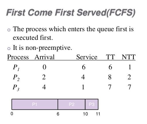
A drawback of the FCFS algorithm is that the processes may have to wait for excessively long amounts of time.

Example

Suppose that there are three processes that arrive in the order shown below. They all arrive at time 0,  but the system has decided to serve them in this order.

Process name	Start time	Burst time
Process 1	0	24
Process 2	0	3
Process 3	0	3

Gantt Cart for FCFS Example

If the processes are served in FCFS order, the Gantt chart would look like as follows:

Process 1

Process 2

Process 3

0                                                              24                                                           27                                                           30

Process 1 is dispatched first and runs for 24-time units (there is no preemption). Once process 1 has finished, process 2 is dispatched and runs for 3-time units.

24-time units have already elapsed, so process 2 starts at time 24. Once process 2 has finished at time 27, the process is dispatched. When process 3 has finished there have been 30-time units used (24+3+3).

The waiting time for a particular process can be measured by taking its finish time and subtracting the burst time and its arrival time. The following table shows the waiting time for each process:

Process name	Arrival time	Burst time	Finish time	Waiting time
Process 1	0	24	24	0
Process 2	0	3	27	24
Process 3	0	3	30	27

Waiting time = finish time – burst time – arrival time

The average waiting time for a whole set of processes can be calculated by adding all the individual waiting times and dividing by the number of processes. In the above example, the average waiting time is : (0+24+27)/ 3 = 17.

Shortest Job First Scheduling Algorithm

Another way to schedule jobs is to pick the job that will take the least amount of time to complete. In FCFS scheduling, the average waiting time could be reduced by running the short jobs first.

The SJF scheduling, the average waiting time could be reduced by running the short jobs first. The SJF scheduling algorithm picks the shortest job in terms of burst size and places it on the CPU.

There are two possible schemes of this scheduling algorithm

• Non- preemptive: once the CPU is given a process it could be preempted until the current CPU burst finishes.
• Preemptive: if a new process arrives with a shorter CPU burst than the remaining CPU burst of the currently executing process, it replaces the currently executing process. It is also called the shortest remaining time first.

Shortest job first scheduling gives the minimum average waiting time for a given set of processes. If you run all the short jobs first, then each subsequent job has a relatively short waiting time. If you were to run all the long jobs first, then every subsequent job would have a longer time to wait.

Non-Preemptive SJF Example

In the following example there are four processes.

Process name	Arrival time	Burst time
Process 1	0	7
Process 2	2	4
Process 3	4	2
Process 4	5	4

 

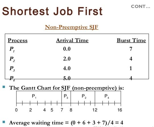
• The arrival times in this example are important. Since there is only 1 process available at time 0 i.e. process 1, it is by default the shortest process.
• At time 2, process 2 arrives but process 1 is already running. There is no preemption, so even though process 2 is now the shortest it has to wait until process 1 finishes.
• At time 4, process 3 arrives which is the shortest but process 1 has still not finished.
• At time 5, process 4 arrives and process 3 is still the shortest. When process 1 finishes, then process 3 will run because it is the shortest.
• When process 3 finishes, process 2 will run. It has the same length as 4 but arrived earlier so we will choose it.
• Finally, process 4 will run.

Gantt Chart for SJF example

Process 1

Process 3

Process 2

Process 4

0                                              7                                              9                                              13                                           17

The waiting times for the processes in this example are:

Process name	Arrival time	Burst time	Finish time	Waiting time
Process 1	0	7	7	0
Process 2	2	4	13	7
Process 3	4	2	9	3
Process 4	5	4	17	8

The average waiting time is : (0 + 9 + 3 + 8) / 4 = 5

Preemptive SJF Example

In the following example, there are again four processes. Note that process 3 now has a burst time of 1.

Process name	Arrival time	Burst time
Process 1	0	7
Process 2	2	4
Process 3	4	1
Process 4	5	4

 

• The arrival times in this example are important. Since there is only 1 process available at time 0 i.e. process 1, it is by default the shortest process.
• At time 2, process 2 arrives, but process 1 is already running. However, there is preemption, so even though process 1 is already running, it is removed from the CPU and replaced with process 2.
• At time 4, process 3 arrives which is now the shortest and it replaces process 2 on CPU.
• At time 5, process 3 finishes, and process 4 arrives. Process 2 is once again the shortest and it gains the CPU, running until time 7.
• At time 7 process 4 is the shortest and runs until time 11.
• Finally, process 1, which is the only process left, is now the shortest and finished.

Gantt chart for SJF example

Process 1

Process 2

Process 3

Process 2

Process 4

Process 1

0                              2                              4                              5                              7                              11                           16

The waiting times for the process in this example are:

Process name	Arrival time	Burst time	Finish time	Waiting time
Process 1	0	7	16	9
Process 2	2	4	7	1
Process 3	4	1	5	0
Process 4	5	4	11	2

The average waiting time is : (9 + 1 + 0 + 2) / 4 =3

Priority Scheduling Algorithm

Another way to schedule jobs is to pick the job that has the highest priority. This requires that each process should have a priority associated with it.

The priority is generally an integer with some well-defined range e.g 1 to 10. The CPU is allocated to the process with the highest priority. In some systems, smaller numbers mean higher priority, in other systems larger numbers mean higher priority.

Priority scheduling can either be non-preemptive or preemptive. If there is preemption then a high-priority job can remove a low-priority job from the CPU and take over.

Non-preemptive example

Process name	Burst time	Priority
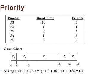
Process 1	10	3
Process 2	1	1
Process 3	2	3
Process 4	1	4
Process 5	5	2

 

Assume that all processes arrived at time 0. First of all, process 2 will get the CPU as it has the highest priority 1 and will finish. Then process 5 will start execution. In non-preemptive priority scheduling, once a process gets the CPU, it will finish its work and then release the CPU.

Gantt chart for Non-preemptive priority scheduling

Process 2

Process 5

Process 1

Process 3

Process 4

0                              1                                              6                                              16                           18                           19

The average waiting time is: (1 + 6 +16 + 18 + 19 ) / 5 =8.2

Preemptive example

Process name	Arrival time	Burst time	Priority
Process 1	0	10	3
Process 2	2	1	1
Process 3	4	2	2
Process 4	6	1	4
Process 5	8	5	5

 

In the above example the execution takes place in the following sequence:

• Process 1 arrives at time 0 and starts execution, as there is no other process.
• At time 2, process 2 arrives with higher priority, so process 1 will be preempted and process 2 will get the CPU and run to the completion using one unit of time at time 3.
• At this point, there is again only one process 1, which resumes and gets the CPU.
• At time 4, process 3 arrives with higher priority than process 1 and gets the CPU and completes its execution.
• At time 6, process 4 arrives with priority 4. Now there are two processes i.e process 1 and process 4. So, process 1 continues using the CPU.
• At time 8, the last process arrives with a priority 5. Process 1 is still a high-priority process, so it will run the completion.
• As P1 releases the CPU after completing its jobs, it will be assigned to p4, which will execute completely.
• In the end, P5 will get the CPU.

Gantt chart for preemptive priority scheduling

P1

P2

P1

P3

P1

P4

P5

0                              2                              3                              4                              6              13                           14           19

Shortest job first scheduling is also a form of priority scheduling. In the case of shortest job scheduling, the priority is defined as the predicted next CPU burst.

One major problem with priority-based scheduling is that it may not be fair. Some low-priority processes may not ever get the chance to execute because higher priority processes keep steeling the CPU. One solution to this problem is to implement aging. The process of increasing the priority of a process as it gets order is known as aging.

Round Robin Algorithm

Another way to schedule jobs is to align a small amount of time to each process in which it executes. The small time unit is usually called the time quantum or time slice.

The job is allocated to the CPU for the time quantum. When the time quantum expires, the process is preempted from the CPU and replaced by the next process in the circular queue.

Example

Process name	Burst time
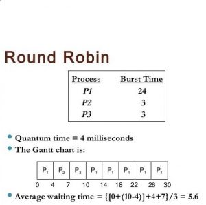
Process 1	24
Process 2	3
Process 3	3

 

Gantt chart for round-robin scheduling

Process 1

Process 2

Process 3

Process 1

Process 1

Process 1

Process 1

Process 1

0              4                              7              10                           14                           18           22                           26           30

Process 1 gets the first 4 units of time. It requires another 20 units so it is preempted after the first time quantum. CPU is given to process 2 that does not require 4 units. It quits before its time quantum ends and the CPU is given to process 3.

Once each process has got a one-time quantum, the CPU is given to process 1 for additional time quantum. Average turnaround time is 47 / 3 = 16.

The round-robin algorithm does not allocate CPU to any process for more than one-time quantum in a row. If CPU burst exceeds time quantum, it is preempted and placed in the ready queue. That is why a round robin is called a preemptive scheduling algorithm.

The round robin scheduling algorithm will be similar to FCFS if the time quantum is very large. If the time quantum is larger than the largest CPU burst for all the processes, then no process will be preempted.

If the time quantum is made too small, then the context switch will take too much time. It is required when preempting one process from the CPU and replacing it with another.

Multi-Level Queue  Algorithm

The previous scheduling algorithms treated different kinds of processes in the same fashion, typically, there is a distinction between interactive processes and non-interactive processes. The interactive processes generally required a much faster response time than non-interactive processes.

These processes can be separated and can be scheduled separately. The interactive processes should be scheduled more quickly than non-interactive processes.

The ready queue can be split into different sub-queues. One sub-queue can be used for each type of process. An example of 5 level queuing strategies is shown below. The 0 has the highest priority and the 4 has the lowest priority.

1. System Processes
2. Interactive Processes.
3. Interactive Editing Processes.
4. Batch Processes.
5. Student Process.

The type of process is automatically identified when it enters the system. It is allocated to the correct queue. There is no way to change queues once a process has been allocated to a queue.

There are five queues in the above example. The individual jobs, as well as five queues, need to be scheduled. Two skills to schedule the queues are as follows:

Fixed (absolute ) Priority

In this scheme, jobs are first serviced 1. If there is no job in queue 1, then the jobs in queue 2 are serviced. Similarly, jobs in queue 3 are all serviced only if there are no jobs in queues 1 or 2 and so on.

Time Slice

In this scheme, each queue gets a time slice. The queues themselves are in a round robin queue. Jobs is each queue are executed for the specified amount of time. The control is then transferred to the next queue.

Multi-Level Feedback Queue Scheduling Algorithm

The main difference between a multi-level queuing strategy and a multi-level feedback queuing strategy is that jobs may move from one queue to another over time.

It is possible to implement aging this way. A process moves up to the next higher priority queue if it stays in one queue too long. The multi-level feedback queue strategy is defined by the following parameters:

• Number of queues
• Scheduling algorithm for each queue
• The method used to determine when to upgrade a process
• The method used to determine when to demote a process
• Method to determine a queue of processes will enter when that process needs service

Example

Suppose there are three queues:

• The Q_0-time quantum 8 milliseconds
• Q_1-time quantum 16 milliseconds
• Q_2-FCFS

The scheduling will be implemented as follows:

A new job enters queue Q_0, which is served FCFS. When it gains CPU, the job receives 8 milliseconds. If it does not finish in 8 milliseconds, the job is moved to queue Q_1. At Q_{1, the} job is again served FCFS and receives 16 additional milliseconds. If it still does not complete, it is preempted and moved to queue Q_2.

Read More:

• CPU Scheduling
• Differences B/w Floppy Disk & Hard Disk